Add Conditional Formatting to Highlight Groups in Excel

Add conditional format highlights groups excel – Add conditional formatting to highlight groups in Excel is a powerful tool that can help you quickly and easily identify patterns and trends in your data. By applying different formatting rules to different groups, you can visually highlight key information and make your spreadsheets more informative and easier to understand.

This technique can be incredibly useful for analyzing data, identifying outliers, and presenting your findings in a clear and concise manner.

Imagine you’re working with a large dataset containing sales figures for different product categories. You want to see which categories are performing well and which are lagging behind. With conditional formatting, you can quickly highlight the top-performing categories in green and the bottom-performing categories in red, making it easy to spot trends and make informed decisions.

Understanding Conditional Formatting

Conditional formatting is a powerful feature in Excel that allows you to automatically change the appearance of cells based on specific criteria. This feature can be used to highlight important data, identify trends, and make your spreadsheets more visually appealing.

Highlighting Groups in Excel, Add conditional format highlights groups excel

Conditional formatting can be used to highlight groups of cells based on specific criteria. This can be useful for identifying trends, analyzing data, and drawing attention to important information. For example, you could highlight all cells in a column that are greater than a certain value, or all cells in a row that contain a specific text string.

Benefits of Using Conditional Formatting for Group Analysis

Conditional formatting offers several benefits for group analysis:

• Improved Visual Clarity:Conditional formatting can help to make your spreadsheets more visually appealing and easier to understand. By highlighting important data, you can quickly identify trends and patterns.
• Enhanced Data Analysis:Conditional formatting can be used to analyze data in a more efficient and effective way. For example, you could use conditional formatting to highlight cells that meet certain criteria, such as being above or below a certain average.
• Increased Productivity:Conditional formatting can save you time and effort by automating the process of highlighting data. This can be particularly helpful when working with large datasets.

“Conditional formatting can be used to quickly identify trends and patterns in your data, making it easier to analyze and interpret.”

Applying Conditional Formatting to Groups

Conditional formatting can be applied to groups of cells, allowing you to highlight specific data patterns within a dataset. This is particularly useful when working with large amounts of data, as it helps to quickly identify trends and anomalies.

Sometimes, when working with large datasets in Excel, it’s helpful to highlight groups of data based on certain criteria. You can use conditional formatting to do this, but sometimes you need to go a step further and visually separate distinct groups.

This is where the power of grouping comes in. Think about how you might want to visually separate different types of sales data, for example, like the way jack wills fed cold rain yet might categorize their product lines.

By grouping and then applying conditional formatting, you can create a clear visual representation of your data that’s easy to understand and analyze. So, whether you’re working with financial reports, sales data, or any other type of spreadsheet, grouping and conditional formatting can be a powerful combination for organizing and highlighting important information.

Applying Conditional Formatting to Groups

To apply conditional formatting to groups of cells, follow these steps:

1. Select the group of cells you want to format.
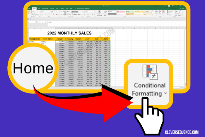
2. Go to the Hometab and click on Conditional Formattingin the Stylesgroup.
3. Select the desired formatting rule from the drop-down menu. You can choose from a variety of pre-defined rules or create your own custom rule.
4. In the New Formatting Ruledialog box, specify the conditions for the rule. This may include things like cell values, dates, or formulas.
5. Select the desired formatting style for the cells that meet the conditions. This could include changing the font color, background color, or adding borders.
6. Click OKto apply the formatting rule.

Using Different Conditional Formatting Rules for Group Highlighting

You can use different conditional formatting rules to highlight different groups within your data. For example, you could highlight cells with values greater than 100 in one color, and cells with values less than 50 in another color.

• To apply multiple rules, follow the steps Artikeld above for each rule. When creating each rule, make sure to select Add Rulefrom the Conditional Formattingmenu. This will add the rule to the existing list of rules.
• The rules will be applied in the order they are listed in the Manage Rulesdialog box. This allows you to prioritize certain rules over others.

Applying Multiple Rules to Highlight Different Groups Simultaneously

You can apply multiple rules to highlight different groups simultaneously. This allows you to highlight multiple data patterns within the same group of cells.

• To apply multiple rules, follow the steps Artikeld above for each rule. When creating each rule, make sure to select Add Rulefrom the Conditional Formattingmenu. This will add the rule to the existing list of rules.
• The rules will be applied in the order they are listed in the Manage Rulesdialog box. This allows you to prioritize certain rules over others.
• For example, you could highlight cells with values greater than 100 in one color, and cells with values less than 50 in another color, and cells with values between 50 and 100 in a third color. This would allow you to quickly identify all three groups of values within your data.

  Sometimes, organizing data in Excel can feel like trying to paint a perfect board and batten wall – you want things to be neat and aligned. Using conditional formatting to highlight groups can be a lifesaver, just like checking out this amazing board and batten bedroom makeover with Arhaus can inspire you to revamp your space.

  With conditional formatting, you can easily identify trends and patterns in your data, which can help you make better decisions.

Advanced Conditional Formatting Techniques

Conditional formatting in Excel is a powerful tool that allows you to highlight cells based on specific criteria. While the basic features of conditional formatting are easy to use, you can also leverage advanced techniques to create more complex and dynamic rules for group highlighting.

Formulas and Custom Rules for Group Highlighting

Formulas and custom rules allow you to create highly specific conditional formatting rules that can be applied to groups of cells based on various criteria. These rules can be used to highlight groups of cells based on values, dates, text, or any combination of these elements.

Sometimes, when working with large datasets in Excel, it’s helpful to highlight groups of data based on certain conditions. This can make it much easier to identify trends or patterns. For example, you might want to highlight all cells in a column that are greater than a certain value.

This can be done using conditional formatting, which is a powerful tool that allows you to apply different formatting rules to cells based on their values. Speaking of powerful tools, I recently came across an article about Hydreight’s announcement of a normal course issuer bid , which could be an interesting development for investors.

Back to Excel, conditional formatting can be used to make your spreadsheets more visually appealing and easier to understand, so it’s definitely worth exploring if you haven’t already.

Here are some examples of how to use formulas and custom rules:

Highlighting groups based on value ranges:

• You can use the formula =A1>100to highlight cells in column A that have values greater than 100.
• You can also use the formula =AND(A1>=100, A1<=200)to highlight cells in column A that have values between 100 and 200.

Highlighting groups based on dates:

• You can use the formula =TODAY()-A1>30to highlight cells in column A that represent dates that are older than 30 days.
• You can also use the formula =MONTH(A1)=12to highlight cells in column A that represent dates in December.

Highlighting groups based on text:

• You can use the formula =ISNUMBER(SEARCH("Approved",A1))to highlight cells in column A that contain the text "Approved."
• You can also use the formula =LEFT(A1,3)="ABC"to highlight cells in column A that start with "ABC."

Highlighting Groups Based on Specific Criteria

Conditional formatting can be used to highlight groups of cells based on various criteria, such as:

• Values:You can highlight groups of cells based on specific values, such as the highest or lowest values in a range, values that fall within a certain range, or values that meet specific criteria. For example, you can highlight all cells in a column that are greater than the average value in that column.

• Dates:You can highlight groups of cells based on specific dates, such as dates that fall within a certain period, dates that are older or newer than a specific date, or dates that meet specific criteria. For example, you can highlight all cells in a column that represent dates in the current month.

• Text:You can highlight groups of cells based on specific text, such as cells that contain specific words or phrases, cells that start or end with specific characters, or cells that meet specific criteria. For example, you can highlight all cells in a column that contain the word "urgent."

Examples of Complex Conditional Formatting Scenarios

Complex conditional formatting scenarios often involve multiple rules and criteria. Here are some examples:

• Highlighting sales targets:You can create a conditional formatting rule that highlights cells in a column representing sales figures based on whether they meet, exceed, or fall short of the target sales figures. This rule can involve multiple conditions and formulas.
• Tracking project deadlines:You can create a conditional formatting rule that highlights cells in a column representing project deadlines based on whether the deadlines are approaching, overdue, or have been met. This rule can involve multiple conditions and formulas, as well as the use of the TODAY() function.

• Analyzing customer data:You can create a conditional formatting rule that highlights groups of customers based on their purchase history, spending habits, or demographics. This rule can involve multiple conditions and formulas, as well as the use of the COUNTIF() and SUMIF() functions.

Practical Applications of Conditional Formatting for Groups

Conditional formatting for groups goes beyond simply highlighting cells; it becomes a powerful tool for uncovering trends, identifying anomalies, and gaining a deeper understanding of your data. This approach allows you to analyze large datasets and make informed decisions based on visual insights.

Identifying Trends Within Different Groups

Conditional formatting can be instrumental in identifying trends within different groups. Imagine you are analyzing sales data for various product categories across different regions. By applying conditional formatting rules, you can highlight cells that show significant increases or decreases in sales compared to previous periods or the overall average.

This visual representation helps you quickly spot regions or product categories that are performing exceptionally well or lagging behind. For instance, you could highlight cells with sales figures that are 20% above or below the average for their respective categories, allowing you to identify potential growth opportunities or areas requiring attention.

Highlighting Outliers or Anomalies

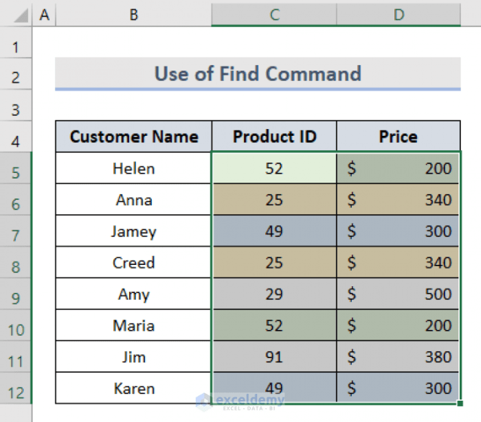
Conditional formatting is highly effective in pinpointing outliers or anomalies within groups. Consider a scenario where you have a dataset containing customer purchase history. By applying conditional formatting rules, you can highlight purchases that deviate significantly from the typical spending patterns of other customers within the same demographic group.

This helps you identify unusual activity, such as potential fraudulent transactions or customers with changing purchasing behaviors. For example, you could highlight purchases that are more than three standard deviations away from the average purchase amount for that customer group.

Improving Data Visualization and Group Analysis

Conditional formatting significantly enhances data visualization and makes group analysis more intuitive. By applying color scales or icons, you can visually represent data trends and patterns, making it easier to grasp complex information at a glance. This visual representation aids in identifying key insights, understanding relationships between groups, and making informed decisions.

For example, you could use a color scale to represent sales performance, with green indicating high performance, yellow indicating average performance, and red indicating low performance. This visual representation allows you to quickly identify the best and worst performing groups and take appropriate actions.

Best Practices for Using Conditional Formatting with Groups: Add Conditional Format Highlights Groups Excel

Conditional formatting is a powerful tool in Excel that allows you to visually highlight data based on specific criteria. When working with groups of data, applying conditional formatting effectively can enhance readability and make it easier to identify trends and patterns.

However, it's crucial to follow best practices to ensure that your conditional formatting is clear, consistent, and effective.

Selecting Appropriate Formatting Styles

Choosing the right formatting styles is essential for creating visually appealing and informative conditional formatting. Consider the following:

• Color Contrast:Select colors that provide sufficient contrast between highlighted and non-highlighted cells. Avoid using colors that are too similar or that clash with the overall spreadsheet design.
• Font Styles:Experiment with font styles like bold, italic, or underline to emphasize certain groups or values. Keep in mind that excessive use of different font styles can make the spreadsheet appear cluttered.
• Fill Patterns:Fill patterns can be helpful for highlighting groups, especially when working with large datasets. Choose patterns that are visually distinct but not distracting.
• Data Bars and Color Scales:Data bars and color scales can be used to visually represent data trends within groups. They provide a quick and easy way to identify high and low values.

Using Clear and Concise Formatting Rules

Clear and concise formatting rules are crucial for avoiding confusion and ensuring that conditional formatting is applied correctly.

• Specific Criteria:Use specific criteria in your formatting rules to ensure that only the desired cells are highlighted. For example, instead of highlighting all cells in a group, highlight only cells that meet a specific condition, such as being above a certain threshold.

• Avoid Ambiguity:Use clear and unambiguous language in your formatting rules. Avoid using jargon or technical terms that may not be understood by everyone who uses the spreadsheet.
• Descriptive Rule Names:Give your formatting rules descriptive names that clearly indicate the purpose of the rule. This will make it easier to understand and manage the formatting rules later on.

Maintaining Consistency and Readability

Consistency and readability are important for creating effective conditional formatting. Consider the following tips:

• Consistent Formatting:Use consistent formatting styles throughout the spreadsheet. This will help to create a visually appealing and organized presentation of data.
• Group Hierarchy:When working with multiple groups, use a hierarchical approach to conditional formatting. This means highlighting the most important groups first, followed by less important groups. This helps to guide the viewer's attention to the most critical information.
• Avoid Overuse:Avoid using too many different conditional formatting rules. This can make the spreadsheet cluttered and difficult to understand. Use conditional formatting strategically to highlight only the most important information.