Microsoft Excel Conditional Formatting: Highlight Rank

Microsoft Excel conditional formatting highlight rank is a powerful tool that can transform your spreadsheets from static data displays into dynamic and visually appealing dashboards. By highlighting ranks, you can quickly identify trends, outliers, and key data points, making it easier to analyze and understand your information.

Whether you’re tracking sales performance, comparing student grades, or analyzing financial data, conditional formatting can be a game-changer.

This technique allows you to apply different colors, patterns, or icons to cells based on their rank within a dataset. For instance, you could highlight the top 10% of sales performers in green, the bottom 10% in red, and everyone else in a neutral color.

This visual representation provides immediate insights and helps you focus on the most important information.

Understanding Conditional Formatting

Conditional formatting in Microsoft Excel is a powerful tool that allows you to automatically change the appearance of cells based on specific criteria. This dynamic formatting can make your spreadsheets more visually appealing and easier to understand.

Highlighting Ranks in Excel

Highlighting ranks in Excel is a specific application of conditional formatting that emphasizes the relative position of data points within a dataset. This can be incredibly useful for quickly identifying top performers, outliers, or trends within your data.

• Identifying Top Performers:When analyzing sales figures, you can use conditional formatting to highlight the top 10% of sales representatives, making it easy to identify and reward high achievers.
• Spotting Outliers:In a dataset of financial data, highlighting values that are significantly higher or lower than the average can help you identify potential errors or anomalies that require further investigation.
• Visualizing Trends:By highlighting data points that fall within certain ranges, you can create visual representations of trends over time. For example, you could highlight sales figures above a certain target to see how performance has improved or declined.

Methods for Highlighting Ranks

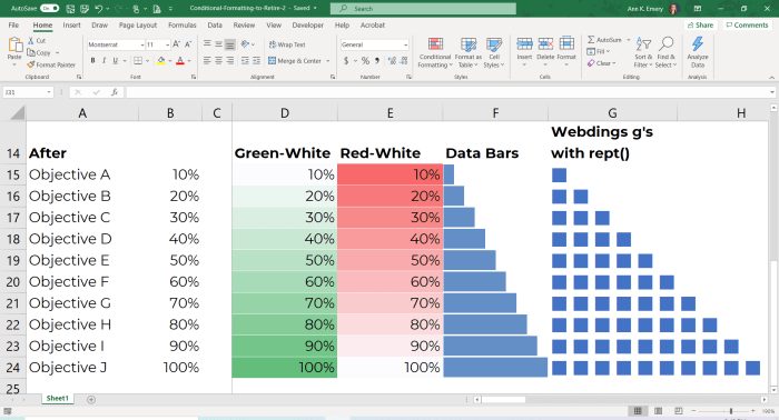
Conditional formatting in Excel provides a powerful way to visually represent data trends and patterns. Highlighting ranks is a common application of conditional formatting, allowing you to quickly identify the top or bottom performers in a dataset. This article explores different methods for highlighting ranks in Excel using conditional formatting.

Sometimes, when I’m working with large datasets in Excel, I find myself using conditional formatting to highlight the top or bottom ranked values. It’s a quick and easy way to spot trends or outliers. This reminded me of the recent news about Hydreight announcing a normal course issuer bid , which could potentially impact their stock price and make it easier to identify significant changes in their share performance.

Back to Excel, though, I find that conditional formatting is a powerful tool for making data analysis more intuitive and efficient.

Using the RANK Function

The RANK function calculates the rank of a value within a dataset. This method allows you to highlight specific ranks based on their position within the dataset.

• Step 1:Select the range of cells you want to apply conditional formatting to.
• Step 2:Go to the “Home” tab and click on “Conditional Formatting” in the “Styles” group.
• Step 3:Select “New Rule” from the dropdown menu.
• Step 4:Choose “Use a formula to determine which cells to format.”
• Step 5:In the “Format values where this formula is true” field, enter the following formula:
  

  =RANK(A1,$A$1:$A$10,0) = 1

  You know how in Microsoft Excel, you can use conditional formatting to highlight the top or bottom ranked cells? It’s like giving your data a little visual boost, making it easier to spot the best or worst performers. And sometimes, just like with Excel, you need a little boost in your life, a chance to connect with your mind and body.

  That’s where the dublin mind body experience comes in, offering a chance to recharge and find balance. So, whether you’re sorting through spreadsheets or sorting through your own thoughts, remember that a little visual or mental clarity can go a long way.

  This formula highlights the cell with the highest value in the selected range. You can modify the formula to highlight other ranks by changing the value on the right side of the equal sign. For example, to highlight the top 3 ranks, use the following formula:

  =RANK(A1,$A$1:$A$10,0) <= 3

• Step 6:Click on the “Format” button and choose the desired formatting style.
• Step 7:Click “OK” to apply the conditional formatting rule.

This method offers flexibility in highlighting specific ranks based on their numerical position within the dataset.

Using the PERCENTILE Function

The PERCENTILE function calculates the value at a specific percentile within a dataset. This method allows you to highlight values based on their relative position within the dataset.

• Step 1:Select the range of cells you want to apply conditional formatting to.
• Step 2:Go to the “Home” tab and click on “Conditional Formatting” in the “Styles” group.
• Step 3:Select “New Rule” from the dropdown menu.
• Step 4:Choose “Use a formula to determine which cells to format.”
• Step 5:In the “Format values where this formula is true” field, enter the following formula:
  

  =A1 >= PERCENTILE($A$1:$A$10,0.9)

  This formula highlights cells with values greater than or equal to the 90th percentile in the selected range. You can adjust the percentile value to highlight different portions of the dataset.

• Step 6:Click on the “Format” button and choose the desired formatting style.
• Step 7:Click “OK” to apply the conditional formatting rule.

This method allows you to highlight a specific percentage of the data, offering a more flexible approach than highlighting specific ranks.

Using the Top/Bottom Rules

Excel provides built-in rules for highlighting top or bottom values. This method offers a simplified approach to highlighting ranks, particularly for quickly identifying the top or bottom performers.

• Step 1:Select the range of cells you want to apply conditional formatting to.
• Step 2:Go to the “Home” tab and click on “Conditional Formatting” in the “Styles” group.
• Step 3:Select “Top/Bottom Rules” from the dropdown menu.
• Step 4:Choose “Top 10 Items” or “Bottom 10 Items.” You can adjust the number of items to be highlighted.
• Step 5:Click on the “Format” button and choose the desired formatting style.
• Step 6:Click “OK” to apply the conditional formatting rule.

This method is a quick and straightforward way to highlight top or bottom values in a dataset, making it a convenient option for basic ranking tasks.

Using the “Greater Than” or “Less Than” Rule

This method allows you to highlight cells based on their comparison to a specific value. It is useful for highlighting values that exceed or fall below a defined threshold.

• Step 1:Select the range of cells you want to apply conditional formatting to.
• Step 2:Go to the “Home” tab and click on “Conditional Formatting” in the “Styles” group.
• Step 3:Select “New Rule” from the dropdown menu.
• Step 4:Choose “Format only cells that contain” from the dropdown menu.
• Step 5:Select “Greater than” or “Less than” from the dropdown menu. Enter the specific value you want to compare to.
• Step 6:Click on the “Format” button and choose the desired formatting style.
• Step 7:Click “OK” to apply the conditional formatting rule.

This method provides a simple way to highlight values that meet specific criteria, making it a versatile option for various ranking scenarios.

Applying Conditional Formatting for Ranks

Conditional formatting in Microsoft Excel is a powerful tool that allows you to visually highlight cells based on specific criteria. This can be particularly useful when working with ranked data, as it enables you to quickly identify the top performers, bottom performers, or specific ranks within your dataset.

Sometimes, when I’m working with data in Excel, I find myself needing to highlight the top or bottom values to quickly identify trends. Conditional formatting is a lifesaver for that, especially when you want to showcase the best-performing products or the lowest-selling items.

It’s almost like creating a visual “cheese board” of data, but instead of fruit and cheese, you’re highlighting the most important data points. Speaking of cheese boards, have you seen this awesome DIY fruit slice cheese board tutorial?

It’s perfect for entertaining friends! Anyway, back to Excel, once you’ve applied the conditional formatting, it’s like having a spotlight on the most crucial data points, making it easier to draw conclusions and make decisions.

Applying Conditional Formatting Rules

To apply conditional formatting rules for ranks, you need to follow these steps:

• Select the cells containing the data you want to rank.
• Go to the “Home” tab and click on “Conditional Formatting” in the “Styles” group.
• Select “New Rule” from the dropdown menu.

Next, you need to choose the type of rule you want to apply. Here are some common scenarios:

Highlighting Top Ranks

• Select “Use a formula to determine which cells to format.”
• In the “Format values where this formula is true” field, enter the formula: =RANK(A1,$A$1:$A$10,0) <= 3. This formula will highlight the top three ranked values in the selected range.
• Click on "Format" to choose the desired formatting style for the highlighted cells.
• Click "OK" to apply the rule.

Highlighting Bottom Ranks

• Select "Use a formula to determine which cells to format."
• In the "Format values where this formula is true" field, enter the formula: =RANK(A1,$A$1:$A$10,0) >= 8. This formula will highlight the bottom two ranked values in the selected range.
• Click on "Format" to choose the desired formatting style for the highlighted cells.
• Click "OK" to apply the rule.

Highlighting Specific Ranks

• Select "Use a formula to determine which cells to format."
• In the "Format values where this formula is true" field, enter the formula: =RANK(A1,$A$1:$A$10,0) = 5. This formula will highlight the fifth ranked value in the selected range.
• Click on "Format" to choose the desired formatting style for the highlighted cells.
• Click "OK" to apply the rule.

Remember to adjust the formula according to your specific requirements, including the cell references, the range of data, and the specific rank you want to highlight.

Advanced Techniques and Customization

Beyond the basic conditional formatting options, Excel offers powerful techniques to customize rank highlighting and achieve more complex results. This section explores advanced methods, including formula-based rules and multi-criteria formatting, to tailor your data visualization to specific needs.

Formulas in Conditional Formatting Rules

Using formulas in conditional formatting rules allows you to apply formatting based on complex calculations or comparisons. This flexibility extends the possibilities beyond simple ranking, enabling you to highlight cells based on various conditions, such as specific values, calculated results, or relationships between cells.

For instance, you could highlight cells where the value is greater than the average of a particular range, or cells where the difference between two columns exceeds a certain threshold.

Here's a breakdown of how to use formulas in conditional formatting:

• Select the range: Choose the cells you want to apply conditional formatting to.
• Open the Conditional Formatting dialog box: Go to the "Home" tab and click on "Conditional Formatting."
• Select "New Rule": Choose "Use a formula to determine which cells to format."
• Enter the formula: In the "Format values where this formula is true" field, type the formula that defines the condition.
• Choose the formatting style: Select the formatting style you want to apply to the cells that meet the formula criteria.

Conditional Formatting Based on Multiple Criteria

Often, you might want to highlight cells based on multiple conditions. Excel allows you to combine multiple criteria using logical operators like "AND" and "OR" within your conditional formatting formulas. This enables you to create more targeted formatting rules.For example, you might want to highlight cells that are both above a certain threshold and within a specific date range.

Here's a sample formula using the "AND" operator:=AND(A1>100,B1>="01/01/2023",B1<="31/12/2023")This formula will format cells in column A if the value is greater than 100 and the corresponding date in column B falls within the year 2023.

You can also use the "OR" operator to apply formatting when at least one of the criteria is met.

For instance, you could highlight cells that are either in the top 10% of the range or below a certain value.

Remember, the "AND" operator requires all conditions to be true for formatting to apply, while the "OR" operator requires at least one condition to be true.

Examples and Use Cases: Microsoft Excel Conditional Formatting Highlight Rank

Conditional formatting to highlight ranks can be incredibly useful in various scenarios, from analyzing sales performance to identifying top-performing students. By visually emphasizing rankings, you can quickly identify trends, outliers, and key insights, facilitating informed decision-making.

Applications in Business

Here are some practical examples of how businesses can leverage conditional formatting to highlight ranks:

• Sales Performance Analysis:Highlight the top 10% of sales representatives based on their monthly revenue. This helps identify high performers and potential areas for improvement within the sales team.
• Customer Segmentation:Rank customers based on their purchase history or lifetime value. This allows businesses to target specific customer segments with tailored marketing campaigns.
• Project Management:Track project progress by ranking tasks based on their completion status or priority. This provides a clear visual representation of project health and potential bottlenecks.

Applications in Education, Microsoft excel conditional formatting highlight rank

Conditional formatting can be effectively used in educational settings to:

• Student Performance Analysis:Highlight students who rank within the top 20% on exams or assignments. This can help identify students who excel and those who might need additional support.
• Class Participation Tracking:Rank students based on their participation in class discussions. This encourages active engagement and provides insights into student engagement levels.
• Grading and Feedback:Use conditional formatting to highlight students who have achieved specific performance criteria, providing visual cues for teachers to quickly identify students who require further attention.

Impact on Data Analysis and Decision-Making

Using conditional formatting to highlight ranks can significantly impact data analysis and decision-making by:

• Improving Data Visualization:Conditional formatting transforms raw data into easily digestible visual representations, making it easier to identify trends, outliers, and key insights.
• Facilitating Quick Analysis:Visual cues provided by conditional formatting allow for rapid analysis and identification of critical information, reducing the time needed to draw conclusions.
• Enhancing Decision-Making:By highlighting key data points, conditional formatting supports informed decision-making by providing a clear visual context for analysis.