

Excel Tips Every User Should Master
Excel Tips Every User Should Master – Are you tired of feeling lost in the vast sea of Excel’s capabilities? Do you wish you could navigate spreadsheets with the ease of a seasoned pro? Well, you’re in luck! This blog post is your guide to mastering essential Excel tips and tricks that will transform you from a spreadsheet novice to a confident data wizard.
Get ready to unlock the hidden power of Excel and streamline your workflow with these game-changing techniques.
From mastering keyboard shortcuts to harnessing the power of formulas and functions, we’ll explore a range of tips that will make your Excel experience smoother and more efficient. We’ll delve into data manipulation techniques that will help you organize, analyze, and extract valuable insights from your spreadsheets.
And we’ll even touch upon the art of visualizing data with charts, allowing you to present your findings in a clear and compelling manner.
Essential Keyboard Shortcuts
Mastering keyboard shortcuts in Excel can significantly boost your productivity. By minimizing mouse clicks and navigating efficiently, you can save valuable time and focus on analyzing your data. Here are five essential keyboard shortcuts every Excel user should know:
Selecting Data Ranges
The “Ctrl + Shift + Arrow Keys” shortcut is a powerful tool for selecting entire data ranges quickly. Here’s how it works:
- Start by selecting the first cell in your data range.
- Press and hold “Ctrl + Shift” and then press the desired arrow key (up, down, left, or right).This will extend the selection to the end of the data range in that direction.
For instance, if you want to select all the cells from A1 to the last row containing data in column A, you would select cell A1, press and hold “Ctrl + Shift,” and then press the down arrow key. The selection will automatically expand to include all cells in column A until it encounters a blank cell.
Editing Cells
The “F2” key provides a convenient way to edit the contents of a cell without having to click on it. This shortcut is especially useful when you need to make quick changes to multiple cells.
Learning a few key Excel tips can really boost your productivity, like using VLOOKUP for quick data searches or mastering pivot tables for insightful analysis. Speaking of mastering, I’m currently obsessing over the Dunnes Stores Joanne Hynes new collection AW Chapter Two – the colors and textures are just incredible! But back to Excel, once you’ve got those basics down, you can really take your spreadsheets to the next level with conditional formatting and data validation.
- Select the cell you want to edit.
- Press the “F2” key.The cell’s contents will become editable, allowing you to make changes directly.
- Press “Enter” to confirm the changes or “Esc” to discard them.
This shortcut eliminates the need to click on the cell to enter edit mode, saving you time and effort.
Mastering Formulas and Functions: Excel Tips Every User Should Master
Formulas and functions are the heart of Excel, allowing you to perform calculations, analyze data, and automate tasks. By understanding how to use them effectively, you can unlock the true power of this spreadsheet software.
Mastering Excel shortcuts can save you hours of time, just like planning your trip to Charleston, South Carolina, can save you from last-minute travel headaches. Check out this comprehensive Charleston South Carolina travel guide for insider tips on the best restaurants, historical sites, and hidden gems.
And while you’re planning your trip, remember to practice those Excel shortcuts so you can create the perfect itinerary in a flash!
Understanding Cell References
Cell references are crucial for creating formulas and functions. They tell Excel which cells to use in your calculations. There are two types of cell references: relative and absolute.
- Relative Cell References: When you copy a formula containing a relative cell reference, the reference adjusts to its new location. For example, if you have the formula “=A1+B1” in cell C1 and copy it to cell C2, the formula will become “=A2+B2” in cell C2.
This is useful for applying the same calculation across multiple cells.
- Absolute Cell References: An absolute cell reference remains constant even when you copy a formula. To make a cell reference absolute, you need to add a dollar sign ($) before the column letter and/or row number. For example, “$A$1” will always refer to cell A1, regardless of where you copy the formula.
This is helpful for referencing specific cells that should not change.
Essential Excel Functions
Here are five commonly used Excel functions that can significantly enhance your data analysis:
- SUM: This function adds a range of numbers. The syntax is “=SUM(number1, [number2], …)”
- AVERAGE: This function calculates the average of a range of numbers. The syntax is “=AVERAGE(number1, [number2], …)”
- IF: This function performs a logical test and returns one value if the test is true and another value if the test is false. The syntax is “=IF(logical_test, [value_if_true], [value_if_false])”
- VLOOKUP: This function searches for a specific value in the first column of a table and returns a corresponding value from another column in the same table. The syntax is “=VLOOKUP(lookup_value, table_array, col_index_num, [range_lookup])”
- COUNTIF: This function counts the number of cells within a range that meet a specified criteria. The syntax is “=COUNTIF(range, criteria)”
Essential Functions for Data Analysis
| Function Name | Description | Syntax | Example |
|---|---|---|---|
| SUM | Adds a range of numbers | =SUM(number1, [number2], …) | =SUM(A1:A5) |
| AVERAGE | Calculates the average of a range of numbers | =AVERAGE(number1, [number2], …) | =AVERAGE(B1:B10) |
| MAX | Returns the largest number in a set of values | =MAX(number1, [number2], …) | =MAX(C1:C20) |
| MIN | Returns the smallest number in a set of values | =MIN(number1, [number2], …) | =MIN(D1:D15) |
| COUNT | Counts the number of cells that contain numbers | =COUNT(value1, [value2], …) | =COUNT(E1:E10) |
| IF | Performs a logical test and returns one value if the test is true and another value if the test is false | =IF(logical_test, [value_if_true], [value_if_false]) | =IF(A1>10, “High”, “Low”) |
| VLOOKUP | Searches for a specific value in the first column of a table and returns a corresponding value from another column in the same table | =VLOOKUP(lookup_value, table_array, col_index_num, [range_lookup]) | =VLOOKUP(A1, B1:C10, 2, FALSE) |
| COUNTIF | Counts the number of cells within a range that meet a specified criteria | =COUNTIF(range, criteria) | =COUNTIF(A1:A10, “>10”) |
Efficient Data Manipulation
Excel offers a variety of tools and functions that make data manipulation a breeze, even for large and complex datasets. This section explores some of the most efficient data manipulation techniques that every Excel user should master.
The Fill Handle
The Fill Handle is a small black square that appears in the bottom right corner of a selected cell. It allows you to quickly copy and paste data, including formulas, across multiple cells. To use the Fill Handle, simply select the cell containing the data you want to copy, hover over the Fill Handle, and drag it down or across to the desired range of cells.
For example, if you have a list of numbers in column A, and you want to copy them to column B, you can select the cells in column A, hover over the Fill Handle, and drag it to column B. Excel will automatically copy the values or formulas to the corresponding cells in column B.
Data Validation
Data Validation is a powerful tool that helps ensure data integrity by preventing users from entering incorrect or invalid data. You can use Data Validation to set rules for specific cells or ranges, such as requiring a specific data type, limiting the number of characters, or restricting values to a predefined list.
Mastering Excel is like mastering a powerful tool, and just like you wouldn’t use a power drill without understanding its safety features, you need to know the essential tips to unlock its full potential. One of the most important skills is using formulas, which can automate repetitive tasks and make your work much more efficient.
And while we’re on the topic of efficiency, have you ever heard the phrase “we got the beet juice”? we got the beet juice is a great example of how a simple phrase can convey a powerful message. Similarly, knowing how to use Excel’s advanced features, like pivot tables and data validation, can give you a significant edge in your work.
So, whether you’re a beginner or a seasoned pro, there’s always something new to learn in the world of Excel.
For example, if you have a column for “Gender,” you can use Data Validation to ensure that only “Male” or “Female” are entered. This prevents users from entering incorrect or inconsistent data, leading to more accurate and reliable data analysis.
Sorting and Filtering
Sorting and filtering are essential tools for organizing and extracting specific data from large datasets. Sorting arranges data in ascending or descending order based on a chosen column, while filtering allows you to display only rows that meet specific criteria.
For example, if you have a list of customer data, you can sort the data by “Last Name” to quickly find a specific customer. You can also filter the data to display only customers who have made purchases in the last month.
- Sorting:To sort data, select the range of cells you want to sort, go to the “Data” tab, and click “Sort.” You can then choose the column to sort by, the sort order (ascending or descending), and whether to include header rows.
- Filtering:To filter data, select the range of cells you want to filter, go to the “Data” tab, and click “Filter.” This will add drop-down arrows to the header row of each column. You can then click the drop-down arrow to select the filter criteria.
Visualizing Data with Charts

Data visualization is a powerful tool for making sense of complex information. Charts transform raw data into easily understandable visual representations, revealing patterns, trends, and insights that might otherwise be missed. Excel offers a wide range of chart types, each designed for specific purposes and data types.
Top 3 Chart Types for Effective Data Visualization
Choosing the right chart type is crucial for effectively communicating your data. Here are three of the most versatile and widely used chart types:
- Bar Charts:Bar charts are excellent for comparing data across categories. They visually represent data as bars, with the height or length of each bar proportional to the value it represents. They are ideal for showing comparisons, trends, and distributions. For instance, you can use a bar chart to compare sales figures for different products or regions over time.
- Line Charts:Line charts are best for visualizing data trends over time. They connect data points with lines, showing how values change over a period. Line charts are useful for identifying patterns, growth, or decline in data, making them ideal for analyzing financial data, website traffic, or sales trends.
- Pie Charts:Pie charts are best for showing the proportions of a whole. They divide a circle into slices, with the size of each slice representing the proportion of a particular category to the whole. Pie charts are effective for visualizing data that adds up to 100%, such as market share, demographics, or budget allocation.
Creating a Simple Bar Chart with Customized Formatting, Excel tips every user should master
Creating a bar chart in Excel is straightforward:
- Select Your Data:Select the range of cells containing the data you want to visualize. This data should include categories (e.g., products, regions) and corresponding values (e.g., sales figures, revenue).
- Insert a Bar Chart:Go to the “Insert” tab in the Excel ribbon and click on the “Bar Chart” icon. Choose the specific bar chart type you want from the drop-down menu. Excel will automatically create a basic bar chart based on your selected data.
- Customize Chart Formatting:Once the chart is created, you can customize its appearance. Click on the chart to select it. You can change the chart title, axis labels, colors, and other formatting options using the “Chart Tools” tab in the Excel ribbon.
- Add Data Labels:To display the exact values on each bar, right-click on a bar and select “Add Data Labels.” You can further customize the appearance of these labels, such as font size, color, and position.
- Adjust Chart Size and Position:Resize the chart by dragging its corners or edges. You can also move the chart to a different location on your spreadsheet.
Chart Types and Their Strengths
| Chart Type | Best Use Cases | Example Data | Key Features |
|---|---|---|---|
| Bar Chart | Comparing data across categories, showing trends, and visualizing distributions | Sales figures for different products, website traffic by region, student grades by subject | Easy to compare data, visually appealing, effective for showing large differences |
| Line Chart | Visualizing data trends over time, showing growth or decline, identifying patterns | Financial data, website traffic, sales trends, temperature fluctuations | Clear visualization of data trends, effective for showing changes over time, ideal for time series data |
| Pie Chart | Showing proportions of a whole, representing data that adds up to 100%, visualizing market share or budget allocation | Market share of different companies, demographic breakdown of a population, budget allocation for different departments | Effective for showing relative proportions, visually appealing, easy to understand |
| Scatter Chart | Showing the relationship between two variables, identifying correlations, visualizing data with outliers | Height and weight of individuals, sales figures and marketing spend, temperature and humidity | Reveals relationships between variables, identifies patterns and outliers, useful for statistical analysis |
| Histogram | Visualizing the distribution of data, showing the frequency of values, identifying patterns and outliers | Distribution of salaries, customer age, product defect rates | Shows data distribution, identifies clusters and gaps, useful for statistical analysis |
Advanced Excel Features
Excel offers a range of advanced features that empower users to analyze data, uncover insights, and make informed decisions. Beyond basic calculations and formatting, these features unlock a new level of efficiency and sophistication in data management.
Pivot Tables
Pivot tables are powerful tools for summarizing and analyzing large datasets. They allow users to quickly create dynamic reports that can be easily filtered, sorted, and grouped to reveal trends and patterns within the data.Pivot tables are particularly useful for:
- Summarizing data: Pivot tables can aggregate data based on specific criteria, such as sales by region, product performance by category, or customer demographics. This allows users to quickly gain a high-level overview of the data.
- Identifying trends: By grouping and filtering data, pivot tables can highlight trends and patterns that might not be immediately apparent in raw data. For example, users can identify peak sales periods, product categories with the highest growth, or customer segments with the highest retention rates.
- Performing calculations: Pivot tables support various calculations, such as sums, averages, counts, and percentages. This allows users to analyze data in different ways and gain deeper insights.
To create a pivot table, users can select the data range and then navigate to the “Insert” tab and choose “PivotTable.” The pivot table wizard will guide users through the process of selecting the data fields and configuring the report layout.
Example:A sales manager can create a pivot table to analyze sales data by region and product category. This would allow them to identify the top-selling products in each region, the regions with the highest sales, and the overall sales performance of each product category.
Data Tables
Data tables are used to explore the impact of changing multiple variables on a specific outcome. They allow users to see how different inputs affect a formula or calculation without manually adjusting each variable.Data tables are beneficial for:
- Sensitivity analysis: Data tables allow users to assess how changes in input variables affect the output of a formula. This can be helpful for understanding the risks and opportunities associated with different scenarios.
- Scenario planning: Data tables can be used to explore different scenarios by changing the values of input variables. This can help users to make informed decisions based on various potential outcomes.
- What-if analysis: Data tables enable users to ask “what if” questions about their data. For example, they can explore the impact of different pricing strategies, marketing campaigns, or production costs on their profitability.
To create a data table, users need to first define the formula or calculation that they want to analyze. Then, they can select a range of cells that will contain the input variables and the corresponding output values. Finally, they can navigate to the “Data” tab and choose “What-If Analysis” > “Data Table.”
Example:A financial analyst can create a data table to explore the impact of different interest rates and loan terms on a mortgage payment. This would allow them to assess the affordability of different loan options and make informed decisions about their financing needs.
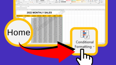
Conditional Formatting
Conditional formatting is a powerful feature that allows users to highlight specific data points based on certain criteria. This can be used to draw attention to trends, outliers, or other important data points within a dataset.Conditional formatting is beneficial for:
- Visualizing data: Conditional formatting can make data more visually appealing and easier to understand. By highlighting specific data points, users can quickly identify trends and patterns.
- Drawing attention to outliers: Conditional formatting can be used to highlight data points that fall outside of a certain range, such as values that are significantly higher or lower than the average. This can help users to identify potential errors or unusual trends.
- Improving data analysis: Conditional formatting can help users to focus on specific data points that are relevant to their analysis. This can save time and effort by eliminating the need to manually search for specific values.
To apply conditional formatting, users can select the data range and then navigate to the “Home” tab and choose “Conditional Formatting.” Excel offers a variety of pre-defined formatting rules, or users can create custom rules based on specific criteria.
Example:A sales manager can apply conditional formatting to highlight sales figures that are above or below a certain target. This would allow them to quickly identify sales teams that are exceeding or falling short of their goals.